In the previous post, we showed Shor’s Algorithm, the theory behind cracking of the RSA using Quantum Computing. In this post, we will show how to program the algorithm using QISKit in order to appreciate how the theory is implemented.

Brief Review of RSA Cryptography
According to the RSA encryption, we choose 2 prime numbers 


If we have a message 

The public only knows about 


Once 

From there, we can finally decrypt our message

Since

Example
Let 


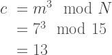
Given only the knowledge of 

Overview of Shor’s Algorithm
We will setup two registers for the Shor’s Algorithm. The first register is the input register. These are the qubits whose value we will input into the modular exponentiation function. The output of that function will be stored in the output register.
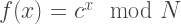
The modular exponentiation function is defined as:
Shor’s algorithm involves:
1. Generating a superposition of all numbers 

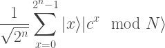
2. We then measure the output register. This will give us a value say 

3. Next, we apply the Fourier Transform to the input register. The Fourier Transform is defined in the computational basis is:

So applying this to the input register will give:

In other words, the input register will become a superposition of states whose probability of occurring is given by the square of the probability amplitude above.
4. We then measure the input register to get a value 
5. Compute the period using the continued fraction expansion of

The fraction 
6. Verify that the computed period is indeed a period by satisfying

7. Compute

where 
8. Use the computed 

Implementation Using QISKit
There are two important circuits we need to create in order to implement Shor’s algorithm. The first is the modular exponentiation and the second is the Fourier Transform. For the modular exponentiation, we are going to implement a similar function that will give the answer specifically to our problem.
The ciphertext we are trying to decrypt is 

If you study the table above, you will notice that for numbers ending in the following suffixes, following mappings are true:

Here is a circuit to implement this mapping:

To verify this, if the input is ends with 00, the output register 


The QISKit code to implement this is:
input_register  = QuantumRegister(4,name="qin")
output_register = QuantumRegister(4,name="qout")

c  = ClassicalRegister(8)
qc = QuantumCircuit(input_register, output_register)
qc.barrier()

qc.x(output_register[0])
qc.barrier()

qc.cx(input_register[0],output_register[2])
qc.cx(input_register[0],output_register[3])
qc.barrier()

qc.cx(input_register[1],output_register[2])
qc.cx(input_register[1],output_register[0])
qc.barrier()

qc.ccx(input_register[0],input_register[1],output_register[3])
qc.ccx(input_register[0],input_register[1],output_register[2])
qc.ccx(input_register[0],input_register[1],output_register[1])
qc.ccx(input_register[0],input_register[1],output_register[0])
qc.barrier()

qc.draw(output='mpl')
Implementing the Fourier Transform
We will use the Fourier Transform circuit derived in this blog post. Here are the sequence of gate operations to implement the Fourier Transform:

where 

Using QISKit, we can visualize the circuit using the code below:
input_register  = QuantumRegister(4,name="qin")
output_register = QuantumRegister(4,name="qout")
c               = ClassicalRegister(4)

qc = QuantumCircuit(input_register,c)
qc.h(input_register[0])
qc.cu1(math.pi/float(2),input_register[0],input_register[1])
qc.cu1(math.pi/float(2**2),input_register[0],input_register[2])
qc.cu1(math.pi/float(2**3),input_register[0],input_register[3])
qc.barrier()

qc.h(input_register[1])
qc.cu1(math.pi/float(2),input_register[1],input_register[2])
qc.cu1(math.pi/float(2**2),input_register[1],input_register[3])
qc.barrier()

qc.h(input_register[2])
qc.cu1(math.pi/float(2),input_register[2],input_register[3])
qc.h(input_register[3])
qc.barrier()
![]()
The Complete Shor’s Algorithm Circuit
Now that we have created the circuits for the “modular exponentiation” and the Fourier Transform, we will combine them to create the circuit for the period finding algorithm.
Here’s the complete code:
from qiskit import Aer

import math

from qiskit import QuantumCircuit, ClassicalRegister, QuantumRegister, execute
from qiskit.tools.visualization import circuit_drawer, plot_histogram
from qiskit import BasicAer

backend = BasicAer.get_backend('qasm_simulator')

input_register  = QuantumRegister(4)
output_register = QuantumRegister(4)
c = ClassicalRegister(8)

qc = QuantumCircuit(input_register, output_register,c)
qc.h(input_register)
qc.barrier()

qc.x(output_register[0])
qc.barrier()

qc.cx(input_register[0],output_register[2])
qc.cx(input_register[0],output_register[3])
qc.barrier()

qc.cx(input_register[1],output_register[2])
qc.cx(input_register[1],output_register[0])
qc.barrier()

qc.ccx(input_register[0],input_register[1],output_register[3])
qc.ccx(input_register[0],input_register[1],output_register[2])
qc.ccx(input_register[0],input_register[1],output_register[1])
qc.ccx(input_register[0],input_register[1],output_register[0])
qc.barrier()

# measure the output
qc.measure([4,5,6,7],[4,5,6,7])
qc.barrier()


#Apply the Fourier Transform to the new state of the input register.
qc.h(input_register[0])
qc.cu1(math.pi/float(2),input_register[0],input_register[1])
qc.cu1(math.pi/float(2**2),input_register[0],input_register[2])
qc.cu1(math.pi/float(2**3),input_register[0],input_register[3])
qc.barrier()

qc.h(input_register[1])
qc.cu1(math.pi/float(2),input_register[1],input_register[2])
qc.cu1(math.pi/float(2**2),input_register[1],input_register[3])
qc.barrier()

qc.h(input_register[2])
qc.cu1(math.pi/float(2),input_register[2],input_register[3])
qc.h(input_register[3])
qc.barrier()

qc.measure([0,1,2,3],[0,1,2,3])

qc.draw(output='mpl')
We then execute this code 1000 times in order to get the probability distributions.
job = execute(qc, backend,shots=1000)
result=job.result()
counts= result.get_counts(qc)
print(counts)
plot_histogram(data=counts, figsize=(14,10))

Interpreting the Result
The count of the resulting states can be printed using
print(counts)
In one of the runs, this is the result we got:
{'01111010': 7, '11010000': 66, '11010011': 7, '00010111': 3, '01000010': 35, '11010110': 1, '11011011': 5, '11010001': 30, '01110101': 1, '01111101': 6, '01110111': 2, '01000001': 42, '11010101': 2, '11011001': 1, '00010011': 7, '11011101': 9, '01001110': 23, '01001111': 63, '01110011': 9, '00011111': 55, '00011110': 22, '00010000': 61, '11010111': 3, '01110000': 57, '01110001': 55, '01110010': 28, '01000110': 4, '00010010': 18, '00010001': 56, '00010101': 3, '00011001': 4, '00011010': 5, '11011110': 35, '00010110': 5, '01001010': 6, '00011101': 8, '11011010': 1, '01001001': 2, '11010010': 26, '01111111': 55, '00011011': 4, '01000101': 3, '01001011': 4, '01000011': 6, '01000000': 60, '01001101': 2, '01111110': 25, '11011111': 57, '01111001': 4, '01110110': 7}
The important qubits to look at are the input qubits. Remember that the qubits are represented from the right to left. So the input qubits are the 4 qubits at the right-most, where the first input qubit is the right-most qubit.
For example, in the result 01111101, the input qubits are the 4 qubits at the right-most:

For this result, the input qubits are 1101. However, because of the design of the Fourier Transform, the order of the qubits are actually reversed and should be 1011, which correspond to the decimal number 11.
Here is a python script shor_expt.py that will make the output easier to read. It will output the count, together with the reversed order of the qubits and the decimal equivalent:
x={'01111010': 7, '11010000': 66, '11010011': 7, '00010111': 3, '01000010': 35, '11010110': 1, '11011011': 5, '11010001': 30, '01110101': 1, '01111101': 6, '01110111': 2, '01000001': 42, '11010101': 2, '11011001': 1, '00010011': 7, '11011101': 9, '01001110': 23, '01001111': 63, '01110011': 9, '00011111': 55, '00011110': 22, '00010000': 61, '11010111': 3, '01110000': 57, '01110001': 55, '01110010': 28, '01000110': 4, '00010010': 18, '00010001': 56, '00010101': 3, '00011001': 4, '00011010': 5, '11011110': 35, '00010110': 5, '01001010': 6, '00011101': 8, '11011010': 1, '01001001': 2, '11010010': 26, '01111111': 55, '00011011': 4, '01000101': 3, '01001011': 4, '01000011': 6, '01000000': 60, '01001101': 2, '01111110': 25, '11011111': 57, '01111001': 4, '01110110': 7}


for k in x.keys():
  h=k[4:]
  hrev = h[::-1]
  sum = 0
  for i in range(0,4):
    sum += pow(2,3-i)*int(hrev[i])

  print("%s %s %s %2d %2d" % ( k, h, hrev, sum, x[k]))
Running this script and sorting the result, we get:
$ python shor_expt.py|sort -r -k 5

11010000 0000 0000  0 66
01001111 1111 1111 15 63
00010000 0000 0000  0 61
01000000 0000 0000  0 60
11011111 1111 1111 15 57
01110000 0000 0000  0 57
00010001 0001 1000  8 56
01111111 1111 1111 15 55
01110001 0001 1000  8 55
00011111 1111 1111 15 55
01000001 0001 1000  8 42
The last column is the count and the column before that is the number 
Computing the Period
Now that we have a 
![\begin{array}{rl} \displaystyle \frac{y}{2^n} &= \displaystyle \frac{15}{2^4} \\[10px] &= \displaystyle \frac{15}{16}\\[10px] &= \displaystyle \frac{1}{1+\displaystyle \frac{1}{15}} \end{array}](https://s0.wp.com/latex.php?latex=%5Cbegin%7Barray%7D%7Brl%7D++%5Cdisplaystyle+%5Cfrac%7By%7D%7B2%5En%7D+%26%3D+%5Cdisplaystyle+%5Cfrac%7B15%7D%7B2%5E4%7D+%5C%5C%5B10px%5D++%26%3D+%5Cdisplaystyle+%5Cfrac%7B15%7D%7B16%7D%5C%5C%5B10px%5D++%26%3D+%5Cdisplaystyle+%5Cfrac%7B1%7D%7B1%2B%5Cdisplaystyle+%5Cfrac%7B1%7D%7B15%7D%7D++%5Cend%7Barray%7D++++&bg=ffffff&fg=3a3a3a&s=2&c=20201002)
which terminates. So the partial sum is also 
which is indeed a period.
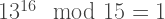
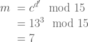
We then compute the inverse modulo using the formula

which will be satisfied if s=5 and 

which is our original message!
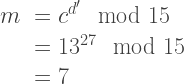
You can verify that if we use 


which gives us the same value.
This completes our implementation of the Shor’s algorithm using QISKit. By implementing the modular exponentiation function as a mapping, we were able to do away with the complexities of a generic modular exponentiation function that will work for any
