Think of a number: How to Program a Quantum Computer

I have always loved figuring out the unknowns. That’s why when I was a child, I love “think of a number” games.

Think of a number, multiply it by 2, add 4, divide the answer by 2. What’s your answer? If your answer is 5, then your number must be 3! The objective is to determine the unknown number.

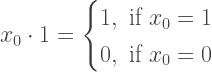
There is a quantum version of this game. First, let’s define an operation called “dot product” of two numbers:
$f(x) = a\cdot x = a_0x_0\oplus a_1x_1\oplus\ldots\oplus a_nx_n$

where $a_i$ is the ith bit of the binary representation of $a$ , and $x_i$ is the i’th bit of $x$ and the symbol $\oplus$ is the XOR operator defined as:

$\begin{array}{rl} 1\oplus 1 &= 0\\ 1\oplus 0 &= 1\\ 0\oplus 1 &= 1\\ 0\oplus 0 &= 0 \end{array}$

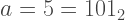
For example, suppose $a=5$ and $x=6$ . The binary representation of $5=101_2$ and the binary representation of $6=110_2$ . Then

$\begin{array}{rl} f(6) &= 1\cdot 1 \oplus 0\cdot 1 \oplus 1\cdot 0\\ &= 1\oplus 0 \oplus 0\\ &= 1 \end{array}$

If you were to guess my number $a$ , how would you go about it?

Well the easiest way to guess my number is to get the dot product of my number with the powers of 2. For example,

$\begin{array}{rl} f(2^0) &= f(1) = 101_2 \cdot 001_2 = 1\\ f(2^1) &= f(2) = 101_2 \cdot 010_2 = 0\\ f(2^2) &= f(4) = 101_2 \cdot 100_2 = 1 \end{array}$

So for an n-bit number, it takes you $n$ invocations of the dot product to determine my hidden number.
The bigger the number, the larger the number of invocations.

Using a quantum computer, it only takes a 1-time invocation of the function in order to guess the number $a$ !

How is it done? You can find how it works from here. In this blog post, we will show how it is implemented using the IBM Quantum Information Science Toolkit.

As we dive into coding, let’s also talk about Quantum Circuits. This is the foundation of programming the quantum computer.

Introducing QISKit

IBM has an opensource framework to program a real Quantum Computer which you can also use to simulate the computation. It’s called QISKit, short for Quantum Information Science Kit. They have an excellent documentation which you can refer for installation instructions.

Assuming we now have installed QISKit, we can start coding our quantum programs. We start with creating some qubits

# Import the Qiskit SDK
from qiskit import QuantumCircuit, ClassicalRegister, QuantumRegister
from qiskit import execute, Aer
from qiskit.tools.visualization import circuit_drawer, plot_histogram

# Create an input Quantum Register with 3 qubits.
qinput = QuantumRegister(3)
# Create an output Quantum Register with 1 qubits.
qoutput= QuantumRegister(1)
# Create a Classical Register with 3 bits.
c = ClassicalRegister(3)
# Create a Quantum Circuit
qc = QuantumCircuit(qinput, qoutput, c)

The most important class in the above code is the QuantumCircuit. This class allows us to perform quantum gate operations on the qubits that we pass to it in the initialization as well as to measure the qubits and write results to the classical qubits.

Quantum Circuits

A circuit is composed of qubits and gates. Gates are operators that act on qubits to change it or to change an output qubit. An example of how we visualize circuits is shown below.

You can see 3 input qubits, 1 output qubit and 3 classical bits. The “meter” icon you see in the drawing indicates that we are measuring the state of the qubit at that point in time and saving the result to a classical qubit.

The code for the above circuit is shown below:

from qiskit import QuantumCircuit, ClassicalRegister, QuantumRegister
from qiskit import execute, Aer
from qiskit.tools.visualization import circuit_drawer, plot_histogram

# Create an input Quantum Register with 3 qubits.
qinput = QuantumRegister(3,name="in")

# Create an output Quantum Register with 1 qubit.
qoutput= QuantumRegister(1,name="out")

# Create a Classical Register with 3 bits.
c = ClassicalRegister(3, name="c")

# Create a Quantum Circuit
qc = QuantumCircuit(qinput, qoutput, c)

The circuit drawing we saw above was easily generated using the following code:

from qiskit.tools.visualization import circuit_drawer

circuit_drawer(qc)

We repeat the output here for convenience:

Measuring the State of the Qubits

Below is the code to measure the input qubits and writing the result to the classical bits. We will execute the circuit 1000 times

shot=1000

and plot the histogram.

qc.measure(qinput, c)

# We will use a simulator
backend_sim = Aer.get_backend('qasm_simulator')
shots = 1000

job_sim = execute(qc, backend=backend_sim, shots=shots)
result_sim = job_sim.result()
answer = result_sim.get_counts()
plot_histogram(answer)

The resulting histogram shows that our qubits are in the initial state of $|000\rangle$ with probability equal to 1.

NOT Gate

By default, our qubits are in the $|0\rangle$ state. To convert it to a $|1\rangle$ qubit, we use the NOT gate:

How do we know that the qubit is indeed in the $|1\rangle$ state? When we measure it, the probability of getting the state $|001\rangle$ is 1. This means if we do the experiment many times, the state will be in $|001\rangle$ all the time!

Below is the result of the measurement:

The Hadamard Gate

Another interesting gate, and in my opinion, is the Hello World of Quantum Computing is the Hadamard gate. The Hadamard gate transforms the basis qubits according to the rule:

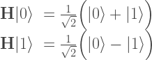
$\begin{array}{rl} \mathbf{H}|0\rangle &= \frac{1}{\sqrt{2}} \Big(|0\rangle + |1\rangle\Big)\\ \mathbf{H}|1\rangle &= \frac{1}{\sqrt{2}} \Big(|0\rangle - |1\rangle\Big)\\ \end{array}$

What makes the Hadamard gate very interesting is that when you apply it to the initial state of

$|\underbrace{000\ldots 0}_{\text{n bit string}}\rangle$ ,

it transforms the initial state into a superposition of all states $|x\rangle$

$\displaystyle \mathbf{H}^{\otimes n} |0\rangle = \displaystyle \frac{1}{\sqrt{2}^n} \sum_{x=0}^{2^{n-1}} |x\rangle$

where

$|x\rangle = |x_{n-1}\rangle\otimes\ldots\otimes|x_2\rangle \otimes|x_1\rangle\otimes|x_0\rangle$ and $x_i \in \{0,1\}$ for $i=0\ldots 2$

Therefore, for $n=3$ , we have a superposition

$|x\rangle = \displaystyle \frac{1}{\sqrt{2}^3} \Big(|0\rangle + |1\rangle + |2\rangle + |3\rangle + |4\rangle + |5\rangle + |6\rangle + |7\rangle\Big)$

Below is a circuit that implements the above superposition:

If we measure the value of $|x\rangle$ , we can see that every state is equally likely to be the value of $|x\rangle$ .

CNOT Gate

The last basic gate we will introduce is the $C_{\mathrm{NOT}}$ gate ( $C_{\mathrm{NOT}}$ stands for Controlled-NOT). The $C_{\mathrm{NOT}}$ gate flips the value of the output qubit depending on the value of the input qubit. It is defined as:

$C_{\mathrm{NOT}}|x\rangle|y\rangle = |x\rangle|y\oplus x\rangle$

Below is an example of a $C_{\mathrm{NOT}}$ circuit.

Here, we flip the value of the first bit using a NOT gate then we apply a $C_{\mathrm{NOT}}$ gate between the first bit and the third bit. Since the first bit is now equal to $|1\rangle$ , the $C_{\mathrm{NOT}}$ will flip the value of the third bit from $|0\rangle$ to $|1\rangle$ . As expected, when we measure the value of the qubits, we find that the state is in $|101\rangle$ with probability equal to 1.

Implementing the Dot Product Circuit

We now have the ingredients that we can use to implement the Dot Product circuit. In this circuit, we have 3 input qubits, 1 output qubit and 3 classical bits. If our hidden number is $a=5$ , this is represented in binary as $101$ . To compute the dot product of any 3 bit number $x$ with $a=5=101_2$ , we draw 3 lines corresponding to the binary representation of $x$ . We also draw the line for the output qubit.

Since $a=101_2$ , the 0th bit of $a$ is 1. Let $x_0$ be the 0th bit of $x$ .

$x_0 \cdot 1 = \begin{cases} 1, \text{ if } x_0 = 1\\ 0, \text{ if } x_0 = 0 \end{cases}$

When $x_0\cdot 1 = 1$ , then it will flip the output qubit. Otherwise, $x_0\cdot 0 = 0$ and it will leave the output qubit as is.

This suggests that we need a $C_\mathrm{NOT}$ gate that connects $|\mathrm{in}_0\rangle$ and $|\mathrm{out}_0\rangle$ .

Therefore,

qc.cx(qinput[0], qoutput[0])

The same is true for $a_2$ :

qc.cx(qinput[2],qoutput[0])

With this in mind, we can program the Dot Product circuit:

from qiskit import QuantumCircuit, ClassicalRegister, QuantumRegister
from qiskit import execute, Aer
from qiskit.tools.visualization import circuit_drawer, plot_histogram

# Create an input Quantum Register with 3 qubits.
qinput = QuantumRegister(3, "in")
# Create an output Quantum Register with 1 qubit.
qoutput= QuantumRegister(1,"out")

# Create a Quantum Circuit
qc = QuantumCircuit(qinput, qoutput)
qc.barrier()
# Add a CX (CNOT) gate on control qubit qinput[0] and target qubit qoutput[0]
qc.cx(qinput[0], qoutput[0])
# Add a CX (CNOT) gate on control qubit qinput[2] and target qubit qoutput[0]
qc.cx(qinput[2],qoutput[0])
qc.barrier()

Finally, Computing for the Unknown Number

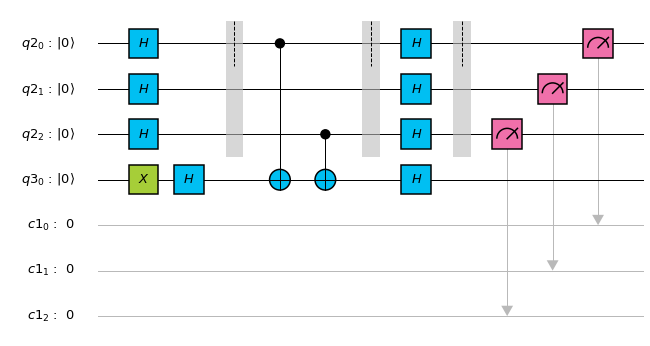
The trick to solving the unknown is by first flipping the output qubit using the NOT gate and applying Hadamards to all qubits:

$\mathbf{H}^{\otimes n+1}\mathbf{U}_f\mathbf{H}^{\otimes n+1}\Big[|0\rangle|1\rangle\Big] = |a\rangle|1\rangle$

See this post for a more detailed explanation.

The circuit corresponding to this equation is the diagram below where we also show barriers that separate the input, the black-box function and the measurement.

The code to do the above is shown below:

from qiskit import QuantumCircuit, ClassicalRegister, QuantumRegister
from qiskit import execute, Aer
from qiskit.tools.visualization import circuit_drawer, plot_histogram

# Create an input Quantum Register with 3 qubits.
qinput = QuantumRegister(3)
# Create an output Quantum Register with 1 qubits.
qoutput= QuantumRegister(1)
# Create a Classical Register with 3 bits.
c = ClassicalRegister(3)
# Create a Quantum Circuit
qc = QuantumCircuit(qinput, qoutput, c)

# Apply Hadamard gate to the input qubits
qc.h(qinput[0])
qc.h(qinput[1])
qc.h(qinput[2])

# Flip the output qubit and apply Hadamard gate.
qc.x(qoutput[0])
qc.h(qoutput[0])

qc.barrier()
# Add a CX (CNOT) gate on control qubit 0 and the output qubit.
qc.cx(qinput[0], qoutput[0])

# Add a CX (CNOT) gate on control qubit 0 and the output qubit.
qc.cx(qinput[2],qoutput[0])

qc.barrier()

# Apply Hadamard gates to all input and output qubits.
qc.h(qinput[0])
qc.h(qinput[1])
qc.h(qinput[2])
qc.h(qoutput[0])


# Add a Measure gate to see the state.
qc.barrier()
qc.measure(qinput, c)

# Compile and use a simulator
backend_sim = Aer.get_backend('qasm_simulator')
shots = 1000

job_sim = execute(qc, backend=backend_sim, shots=shots)
result_sim = job_sim.result()
answer = result_sim.get_counts()
plot_histogram(answer)

# Draw the circuit
from qiskit.tools.visualization import circuit_drawer
my_style = {'plotbarrier': True}
circuit_drawer(qc,style=my_style)

Measuring the state of the input qubits after the computation, we get with probability 1 our hidden number $a=5=101_2$ .

Coloring the Circuits

You might have noticed that our circuit has colors while the code only gives a black-and-white color. To color our circuits, we use the following code:

from qiskit.tools.visualization import matplotlib_circuit_drawer as drawer, qx_color_scheme
my_scheme=qx_color_scheme()
my_scheme['plotbarrier'] = True
drawer(qc, style=my_scheme)

Conclusion

It’s now fairly easy to write quantum programs using IBM QISKit. In the future, it will even be much easier as we will just be using the libraries and composing them in high-level rather than really looking at the algorithms from a low-level. Just as AI is now accessible to a lot of people, Quantum Computing will have it’s day as well.

Spherical Cows In A Vacuum

Thoughts on Mathematics, Physics and Computing

Think of a number: How to Program a Quantum Computer

Introducing QISKit

Quantum Circuits

Measuring the State of the Qubits

NOT Gate

The Hadamard Gate

CNOT Gate

Implementing the Dot Product Circuit

Finally, Computing for the Unknown Number

Coloring the Circuits

Conclusion

Leave a Reply Cancel reply

Think of a number: How to Program a Quantum Computer

Introducing QISKit

Quantum Circuits

Measuring the State of the Qubits

NOT Gate

The Hadamard Gate

CNOT Gate

Implementing the Dot Product Circuit

Finally, Computing for the Unknown Number

Coloring the Circuits

Conclusion

Share this:

Like this:

Related

Leave a Reply Cancel reply